Signal Processing for Steel Drum Leak Detection Based on Time-Frequency Domain (3)

Van Persie

Chapter III: Time-Frequency Analysis of Leakage Acoustic Signals

This paper utilizes MATLAB software to simulate the time-frequency analysis of acoustic emission signals from steel drums. Based on the collected acoustic emission data, the sampling frequency fs is set at 1000 kHz, with a total of 2048 sampling points. The time t is calculated as t = n/fs, where n represents any of the 2048 points, ranging from 0 to N-1. The signals are analyzed in both the time and frequency domains to extract meaningful information about the leakage characteristics.

3.1 Frequency Domain Analysis of Leakage Signals

The acoustic emission signal from a leaking steel drum has a wide frequency spectrum, including components in both audible and ultrasonic ranges. These frequency components may propagate through the leaking drum to the sensor, resulting in a complex spectral composition [1]. As shown in Figure 3.2, a certain leakage signal exists within the frequency range of 0–150 kHz. However, only specific frequency bands are relevant for detecting the leak, while other frequencies may interfere with the detection process. Therefore, it is necessary to process the collected acoustic emission signals to isolate the desired frequency components.

3.1.1 Spectrum Analysis

Fourier transform is a widely used method for analyzing signals, allowing for the decomposition of signal components and their reconstruction [2]. MATLAB offers various functions for fast transformations, such as fft, wewt, fft2, and ift2. Among these, fft2 and ifft2 are two-dimensional fast Fourier transforms for discrete data, while fft and ifft perform one-dimensional fast forward and inverse transformations on discrete data [2]. Since MATLAB does not support zero-based indexing, the subscripts in the formulas are shifted to the right by one.

The acoustic emission signal from the steel drum was subjected to FFT, as shown in Figure 3.1.

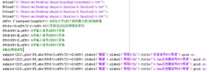
Figure 3.1 FFT Part of the Program Code

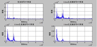
Figure 3.2 Spectrogram of the Acoustic Emission Signal

The waveform in Figure 3.2 is obtained using FFT. Comparing the FFT of the leakage signal with that of a standard signal, the leakage signal shows a significantly higher amplitude around 110 kHz. Additionally, when comparing leakage signals with different aperture sizes, the amplitude around 110 kHz increases as the aperture size increases. This indicates that the characteristic frequency of the acoustic emission signal from a leaking steel drum is approximately 110 kHz, while the noise frequency is around 25 kHz.

3.1.2 Noise Reduction of Leaking Acoustic Emission Signals

The acoustic emission signal from a leaking steel drum passes through multiple stages, including the drum wall, sensor, signal acquisition card, transmission equipment, and amplifier, which introduces significant noise into the signal. This noise can distort the original signal and reduce the accuracy of leak detection. To address this, an appropriate signal processing method must be applied to suppress the noise and enhance the true acoustic emission signal.

Based on the spectrogram obtained from the FFT, the leakage acoustic emission signal exhibits two prominent peaks in the frequency domain: one representing noise and the other corresponding to the characteristic frequency of the signal. Given that the characteristic frequency of the acoustic emission signal is around 110 kHz, we need to filter out high and low frequency components. Since the acoustic emission signal is a non-stationary random signal, a suitable filtering method is the FIR bandpass filter [26].

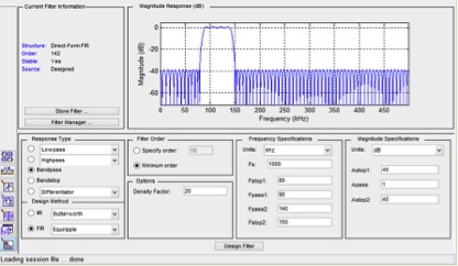
Figure 3.3 FIR Filter Interface

The design uses the MATLAB tool FDATool to create the FIR filter, as shown in Figure 3.3. The filtering process is effectively implemented. Based on the characteristics of the leakage acoustic emission signal and the parameters of the FIR filter [23], the initial design of the amplitude-frequency response is shown in Figure 3.4, and the phase delay diagram is presented in Figure 3.5. The main filter parameters are set as follows: (1) Bandpass response type; (2) Equal ripple design method; (3) Minimum filter order; (4) Density factor of 20; (5) Sampling frequency Fs = 1000 kHz, passband frequencies Fpass1=90kHz and Fpass2=140kHz, stopband frequencies Fstop1=80kHz and Fstop2=150kHz, passband ripple Apass=1dB, stopband attenuation Astop1=40dB, Astop2=40dB.

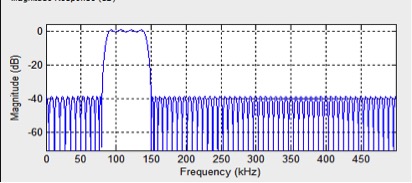
Figure 3.4 Amplitude-Frequency Map

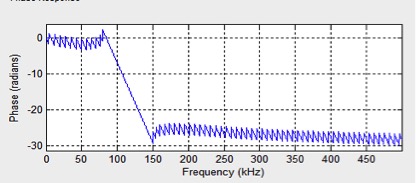
Figure 3.5 Phase Delay Diagram

After designing the filter, the collected acoustic emission signal is filtered using the following steps: open the fdatool interface, select Export, set the output variable name to Num, then assign b=Num and a=1 in the editor, and finally apply the filter using x = filter(b, a, A). The specific code is shown in Figure 3.6. After filtering, the time-domain waveform of the acoustic emission signal is displayed in Figure 3.7.

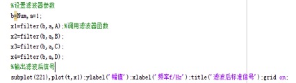
Figure 3.6 Filter Program Part Code

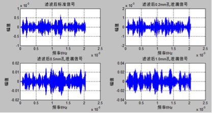
Figure 3.7 Filtered Acoustic Emission Signal Time-Domain Waveform

Comparing the time-domain waveforms before and after filtering, as shown in Figures 3.15 and 3.7, it is evident that the low-frequency noise in Figure 3.7 has been reduced, making the filtered signal more visible. However, some low-frequency interference remains, causing irregular pulses in the filtered signal. Additionally, a small portion of distortion occurs at the beginning of the filtering process due to the filter's delay before full operation [4].

3.1.3 Power Spectrum Estimation

The purpose of power spectrum estimation is to describe the frequency component distribution of a signal and a random process based on finite data. The power spectrum of the filtered acoustic emission signal from the steel drum is shown in Figure 3.9. The specific procedure is illustrated in Figure 3.8.

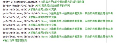
Figure 3.8 Power Spectrum Estimation Partial Program Code

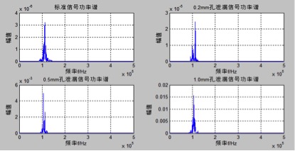
Figure 3.9 Acoustic Emission Signal Power Spectral Density

Based on the power spectrum estimation analysis of acoustic emission signals from multiple groups of steel drums, the amplitude of the power spectral density increases with the size of the leakage aperture. The maximum spectral density of the standard steel drum is around 310–6. If the maximum power spectral density of the acoustic emission signal exceeds 110–5, it suggests that the steel drum is likely to be leaking.

3.1.4 Hilbert-Huang Transform (HHT)

The Hilbert-Huang Transform captures the local characteristics of the acoustic emission signal and decomposes it into intrinsic mode functions (IMFs), revealing different scales of the signal. The IMF represents the intrinsic fluctuation mode of the acoustic emission signal. Analyzing the IMFs after empirical mode decomposition yields rich time-frequency energy information, as shown in Figure 3.10. Empirical mode decomposition is performed on the acoustic emission signal collected under a 0.5 mm aperture leakage condition. The decomposition pattern is shown in Figure 3.11, and the results are analyzed using Hilbert spectrum and marginal spectrum analysis.

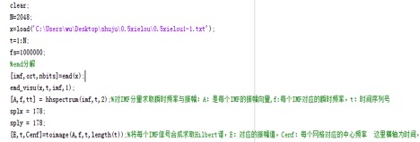
Figure 3.10 Empirical Mode Decomposition Partial Program Code

As shown in Figure 3.11, seven natural mode functions are obtained through empirical mode decomposition. After detailed analysis, the first IMF corresponds to the leakage acoustic emission signal, while the second IMF represents a noise signal at around 25 kHz. The seventh IMF corresponds to the smallest characteristic component of the acoustic emission signal for the steel drum leakage.

Figure 3.11 Empirical Mode Decomposition of the Leakage Signal

Applying the Hilbert transform to the intrinsic mode function obtained from the empirical mode decomposition of the leakage signal in Figure 3.11 produces the Hilbert spectrum shown in Figure 3.12 and the marginal spectrum shown in Figure 3.13. Both spectra reveal signal frequencies around 25 kHz and 110 kHz. According to earlier analysis, the signal near 25 kHz is noise, while the leakage acoustic emission signal is centered around 110 kHz. The energy of the signal is obtained through the Hilbert transform of the acoustic emission signals from steel drums with different apertures. The larger the leakage aperture, the greater the energy of the marginal spectrum.

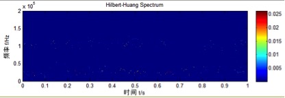
Figure 3.12 Leakage Signal Hilbert Spectrum

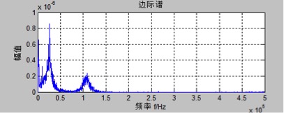
Figure 3.13 Leakage Signal Marginal Spectrum

By comparing the marginal spectrum analysis of filtered acoustic emission signal data from multiple sets of standard steel drums and those with different leakage apertures, it is observed that the maximum marginal spectrum of the standard steel drum acoustic emission signal is less than 1.3. If the marginal spectrum of the acoustic emission signal exceeds 1.3, it indicates that the steel drum is leaking.

3.2 Time Domain Analysis of Leakage Signals

3.2.1 Time Domain Simulation Waveforms and Their Distribution

From the time-domain waveform of the acoustic emission signal, it can be observed that the amplitude characteristics of the steel drum leakage signal change over time as the leakage aperture changes. Thus, the amplitude variation can be visualized in the time-domain simulation waveform. During the actual detection process of steel drum leakage, the acoustic emission signal from the leakage source is usually weak, so it is amplified by an amplification circuit, converted into digital data, and then input into the computer for analysis. As shown in Figure 3.14, the standard signal, 0.2 mm aperture leakage signal, 0.5 mm aperture leakage signal, and 1.0 mm aperture leakage signal data are labeled as ABCD and plotted, with time on the x-axis and amplitude on the y-axis. The program execution results are shown in Figure 3.15.

As seen in Figure 3.15, the simulated time-domain waveform of the leakage acoustic emission signal provides an approximate view of the amplitude changes but lacks detailed description and analysis. To obtain the time-domain characteristic parameters of the leakage acoustic emission signal, further quantitative analysis is required.

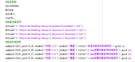
Figure 3.14 Drawing Time-Domain Waveform Program

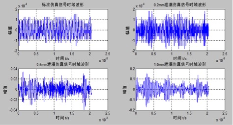
Figure 3.15 Steel Drum Acoustic Emission Signal Time-Domain Waveform

To better analyze the time-domain characteristic parameters of the leakage acoustic emission signal, the acoustic emission signals from the leaking steel drums are divided into five groups based on the standard steel drum and different aperture sizes. The amplitudes of each group are recorded, and a table is created to analyze the signal amplitude characteristics.

Table 3.1 Relationship Between Leakage Aperture Size and Amplitude

It can be observed from Table 3.1 that when the pressure inside the steel drum is constant, the larger the leakage aperture, the higher the amplitude of the acoustic emission signal.

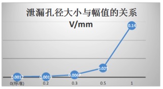
Figure 3.16 Relationship Between Leakage Aperture Size and Amplitude

By connecting the coordinates of the points in Table 3.1 sequentially, the amplitude distribution curves of the leakage signals for the standard steel drum and those with different leakage apertures can be drawn, as shown in Figure 3.16. The figure illustrates that the leakage acoustic emission signal varies depending on the acoustic emission source. When the leakage aperture is large, the amplitude of the acoustic emission signal is more dispersed, with a larger difference between positive and negative amplitudes. Conversely, when the leakage aperture is small or absent, the amplitude of the acoustic emission signal is more concentrated, with a smaller peak-to-peak amplitude. This demonstrates that the amplitude distribution of the leakage signal is closely related to the size of the leakage aperture.

3.2.2 Mean (SAL) and Mean Square (RMS) of Acoustic Emission Time Domain Signals

Analyzing the time-domain characteristic parameters of random signals is an effective way to describe them. The time-domain parameters of acoustic emission signals include mean value, root mean square (RMS), and variance. Experiments were conducted on standard steel drums, as well as those with 0.2 mm, 0.5 mm, and 1.0 mm leakage apertures, with five trials per group. The procedure is shown in Figure 3.17. As presented in Table 3.2, the RMS and mean values of several sets of filtered acoustic emission signals are obtained.

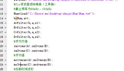
Figure 3.17 Finding the Mean Value Partial Program

Table 3.2 Calculation Results of Time-Domain Feature Quantities of Leakage Signal

As shown in Table 3.2, the mean value does not reflect the characteristics of the leakage source. However, the mean square value shows a consistent trend across repeated tests for the same leakage aperture. Moreover, the mean square value increases as the leakage aperture size increases, indicating that it can be used as an indicator to determine the size of the leak in practical applications.

3.3 Summary of This Chapter

This chapter details the characteristics and processing methods of the leakage signal, focusing on the time domain mean square value, fast Fourier transform, power spectrum, and Hilbert transform. Using a self-developed steel drum leakage acoustic emission signal detection system, the acoustic emission signal of the steel drum is analyzed and processed. The analysis results of the filtered leakage signal are summarized in the following table:

Table 3.3 Signal Characteristic Parameters of Different Leakage Apertures

According to Table 3.3, the frequency domain characteristic parameters and the mean square value of the leakage acoustic emission signal increase as the leakage aperture of the steel drum increases.

[1] Jiang Tao. Application research on pipeline leak detection and location [D]. Harbin Engineering University, 2008. [2] Yang Lijuan, Zhang Baihua, Ye Xuyu. Fast Fourier Transform FFT and its application [J]. Photoelectric Engineering, 2004, 31 (supplement): 1–7. [3] Hu Liying, Xiao Peng. Application of fast Fourier transform in spectrum analysis [J]. Journal of Fujian Normal University (Natural Science Edition), 2011 (04). [4] Song Aiguo, Liu Wenbo, etc. Test signal analysis and processing [M]. Mechanical Industry Press, 2007. [5] Huang Zhenfeng, Wu Jiangjun, Mao Hanling. Filter parameter setting method for metal crack acoustic emission signal FIR filter design [J]. Journal of Hebei University of Technology, 2007 (01): 36. [6] Yu Hao. Research on acoustic emission technology (AE) monitoring system for oil pipeline leakage [D]. Xi'an University of Science and Technology, 2009. 【Related Links】 Steel drum leakage detection signal processing based on time-frequency domain (1) Steel drum leakage detection signal processing based on time-frequency domain (2) Steel drum leakage detection signal processing based on time-frequency domain (3) Steel drum leakage detection signal processing based on time-frequency domain (4) Steel drum leakage detection signal processing based on time-frequency domain (5)

Biodegradable Shopping Bags

All 100% biodegradable shopping bag can be fully degraded, and have passed the American ASTM-D6400 and EU EN13432 compostable certification Standard test. Our biodegradablebag products are made of 100% biodegradable resin as raw materials, free of plastic, non-toxic and harmless.

Bury the used biodegradable bags in the soil, or bury them in the environment with microorganisms. The compost can degrade 100% into carbon dioxide and water in 3 months and become organic fertilizer without white pollution.

Biodegradable T Shirt Bags,Biodegradable Plastic Shopping ,Compostable Grocery Bags,Biodegradable Plastic Grocery Bags

Shaoxing Greenstar New Material Co.,Ltd , https://www.greenstarpackage.com